Screenshots: Unterschied zwischen den Versionen
Dirk (Diskussion | Beiträge) (Created page with "== The Main Window == After starting OpenOpal, the main '''GUI''' appears (Fig. 1). The figure contains an example for an optimization using 4 '''Module'''s. Each module has a...") |
Admin (Diskussion | Beiträge) |
||
| (5 dazwischenliegende Versionen von 2 Benutzern werden nicht angezeigt) | |||
| Zeile 1: | Zeile 1: | ||
== The Main Window == | == The Main Window == | ||
| − | After starting | + | After starting software, the main '''GUI''' appears (Fig. 1). The figure contains an example for an optimization using 4 '''Module'''s. Each module has a name and an unique ID. The software is strictly modular. All functionality for automated optimization and machine learning is encoded in the modules. Here: |
Module 1 (<code>OptAlgCMA</code>) is an optimization algorithm. It is connected via Module 3 (<code>Protocoller</code>) with Module 2 (<code>ProblemSimple</code>). Module 2 contains the optimization problem, i.e. the function to minimize. Here, it is a simple continuous, quadratic function. | Module 1 (<code>OptAlgCMA</code>) is an optimization algorithm. It is connected via Module 3 (<code>Protocoller</code>) with Module 2 (<code>ProblemSimple</code>). Module 2 contains the optimization problem, i.e. the function to minimize. Here, it is a simple continuous, quadratic function. | ||
Module 3 (<code>Protocoller</code>) is a protocoling module, i.e. it stores all evaluated solutions of an optimization run. These solutions can be visualized with Module 4 (<code>DataViewer</code>). | Module 3 (<code>Protocoller</code>) is a protocoling module, i.e. it stores all evaluated solutions of an optimization run. These solutions can be visualized with Module 4 (<code>DataViewer</code>). | ||
| − | [[Image: | + | [[Image:MainGUI.png|frame|center|Figure 1: Main GUI of OpenDino]] |
== Adding, Editing, and Connecting Modules == | == Adding, Editing, and Connecting Modules == | ||
| Zeile 16: | Zeile 16: | ||
In Fig. 2, the right-click is made on Module 4, e.g. for setting the options of this module. | In Fig. 2, the right-click is made on Module 4, e.g. for setting the options of this module. | ||
| − | [[Image: | + | [[Image:ModuleRightclick.png|frame|center|Figure 2: Editing Modules]] |
== Running an Optimization == | == Running an Optimization == | ||
| Zeile 22: | Zeile 22: | ||
Right-clicking Module 1 and selecting the option <code>Run</code> starts an optimization. The standard output of the optimization is given in the lower part of the main window in Fig. 3. | Right-clicking Module 1 and selecting the option <code>Run</code> starts an optimization. The standard output of the optimization is given in the lower part of the main window in Fig. 3. | ||
| − | [[Image: | + | [[Image:Optimization.png|frame|center|Figure 3: Running an Optimization]] |
== Postprocessing an Optimization == | == Postprocessing an Optimization == | ||
| Zeile 28: | Zeile 28: | ||
Right-clicking Module 4 and selecting the option <code>Run</code> starts an the data viewer. Figure 4 shows the evolution of the objective function ''f'' over the number of evaluations. As the objective function is a simple quadratic function (x^2), the minimal function value is zero, which is approximated by 1e-12. | Right-clicking Module 4 and selecting the option <code>Run</code> starts an the data viewer. Figure 4 shows the evolution of the objective function ''f'' over the number of evaluations. As the objective function is a simple quadratic function (x^2), the minimal function value is zero, which is approximated by 1e-12. | ||
| − | [[Image: | + | [[Image:DataViewer.png|frame|center|Figure 4: Postprocessing an Optimization with the DataViewer module. ]] |
| − | |||
| − | |||
| − | |||
| − | |||
Aktuelle Version vom 7. April 2019, 13:29 Uhr
Inhaltsverzeichnis
The Main Window
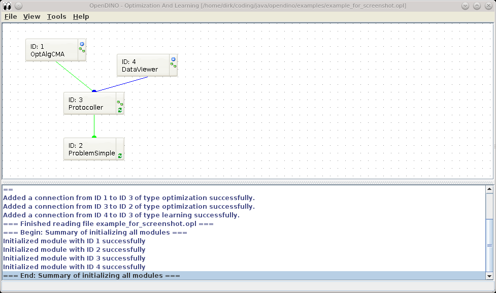
After starting software, the main GUI appears (Fig. 1). The figure contains an example for an optimization using 4 Modules. Each module has a name and an unique ID. The software is strictly modular. All functionality for automated optimization and machine learning is encoded in the modules. Here:
Module 1 (OptAlgCMA) is an optimization algorithm. It is connected via Module 3 (Protocoller) with Module 2 (ProblemSimple). Module 2 contains the optimization problem, i.e. the function to minimize. Here, it is a simple continuous, quadratic function.
Module 3 (Protocoller) is a protocoling module, i.e. it stores all evaluated solutions of an optimization run. These solutions can be visualized with Module 4 (DataViewer).
Adding, Editing, and Connecting Modules
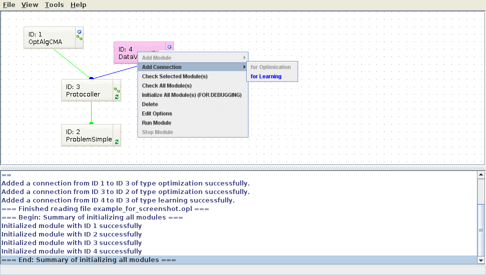
Right-clicking on the dotted area or on a module opens a dialogue as shown in Fig. 2. This dialogue supports:
- adding modules (if clicked on a free space)
- removing modules or changing the options of a module when clicking on a module
- adding/removing connections between modules
- checking and running modules
In Fig. 2, the right-click is made on Module 4, e.g. for setting the options of this module.
Running an Optimization
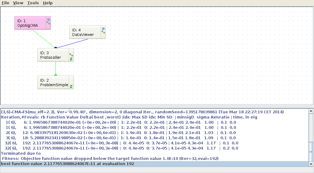
Right-clicking Module 1 and selecting the option Run starts an optimization. The standard output of the optimization is given in the lower part of the main window in Fig. 3.
Postprocessing an Optimization
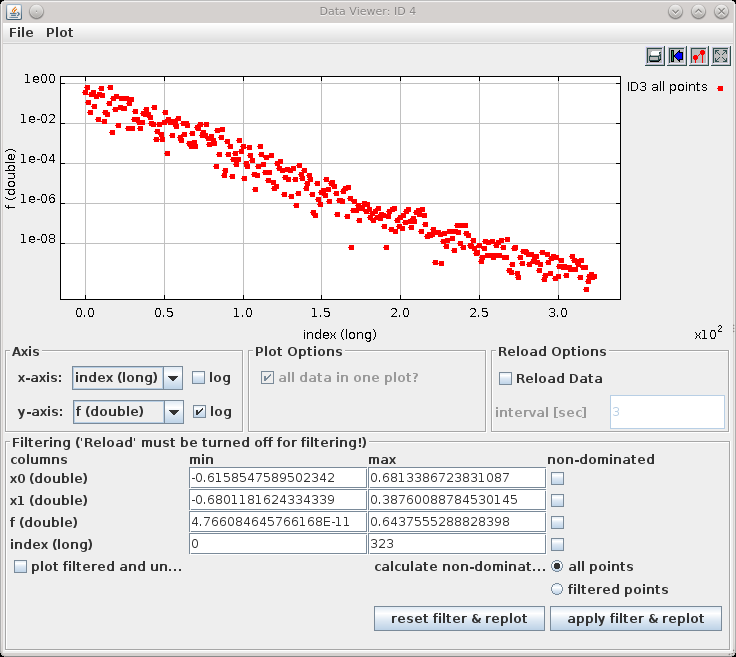
Right-clicking Module 4 and selecting the option Run starts an the data viewer. Figure 4 shows the evolution of the objective function f over the number of evaluations. As the objective function is a simple quadratic function (x^2), the minimal function value is zero, which is approximated by 1e-12.


